# RVM-MATLAB
**Repository Path**: gshang/RVM-MATLAB
## Basic Information
- **Project Name**: RVM-MATLAB
- **Description**: No description available
- **Primary Language**: Unknown
- **License**: Not specified
- **Default Branch**: master
- **Homepage**: None
- **GVP Project**: No
## Statistics
- **Stars**: 0
- **Forks**: 0
- **Created**: 2022-02-06
- **Last Updated**: 2022-02-06
## Categories & Tags
**Categories**: Uncategorized
**Tags**: None
## README
Relevance Vector Machine (RVM)
MATLAB code for Relevance Vector Machine
Version 2.1, 31-AUG-2021
Email: iqiukp@outlook.com
## Main features
- RVM model for binary classification (RVC) or regression (RVR)
- Multiple kinds of kernel functions (linear, gaussian, polynomial, sigmoid, laplacian)
- Hybrid kernel functions (K =w1×K1+w2×K2+...+wn×Kn)
- Parameter Optimization using Bayesian optimization, Genetic Algorithm, and Particle Swarm Optimization
## Notices
- This version of the code is not compatible with the versions lower than R2016b.
- Detailed applications please see the demonstrations.
- This code is for reference only.
## Citation
```
@article{tipping2001sparse,
title={Sparse Bayesian learning and the relevance vector machine},
author={Tipping, Michael E},
journal={Journal of machine learning research},
volume={1},
number={Jun},
pages={211--244},
year={2001}
}
```
```
@article{qiu2021soft,
title={Soft sensor development based on kernel dynamic time warping and a relevant vector machine for unequal-length batch processes},
author={Qiu, Kepeng and Wang, Jianlin and Wang, Rutong and Guo, Yongqi and Zhao, Liqiang},
journal={Expert Systems with Applications},
volume={182},
pages={115223},
year={2021},
publisher={Elsevier}
}
```
## How to use
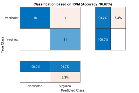
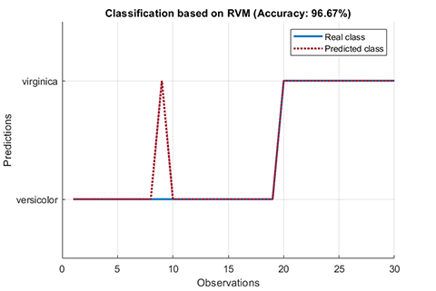
### 01. Classification using RVM (RVC)
A demo for classification using RVM
```
clc
clear all
close all
addpath(genpath(pwd))
% use fisheriris dataset
load fisheriris
inds = ~strcmp(species, 'setosa');
data_ = meas(inds, 3:4);
label_ = species(inds);
cvIndices = crossvalind('HoldOut', length(data_), 0.3);
trainData = data_(cvIndices, :);
trainLabel = label_(cvIndices, :);
testData = data_(~cvIndices, :);
testLabel = label_(~cvIndices, :);
% kernel function
kernel = Kernel('type', 'gaussian', 'gamma', 0.2);
% parameter
parameter = struct( 'display', 'on',...
'type', 'RVC',...
'kernelFunc', kernel);
rvm = BaseRVM(parameter);
% RVM model training, testing, and visualization
rvm.train(trainData, trainLabel);
results = rvm.test(testData, testLabel);
rvm.draw(results)
```
results:
```
*** RVM model (classification) train finished ***
running time = 0.1604 seconds
iterations = 20
number of samples = 70
number of RVs = 2
ratio of RVs = 2.8571%
accuracy = 94.2857%
*** RVM model (classification) test finished ***
running time = 0.0197 seconds
number of samples = 30
accuracy = 96.6667%
```
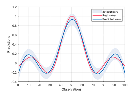
### 02. Regression using RVM (RVR)
A demo for regression using RVM
```
clc
clear all
close all
addpath(genpath(pwd))
% sinc funciton
load sinc_data
trainData = x;
trainLabel = y;
testData = xt;
testLabel = yt;
% kernel function
kernel = Kernel('type', 'gaussian', 'gamma', 0.1);
% parameter
parameter = struct( 'display', 'on',...
'type', 'RVR',...
'kernelFunc', kernel);
rvm = BaseRVM(parameter);
% RVM model training, testing, and visualization
rvm.train(trainData, trainLabel);
results = rvm.test(testData, testLabel);
rvm.draw(results)
```
results:
```
*** RVM model (regression) train finished ***
running time = 0.1757 seconds
iterations = 76
number of samples = 100
number of RVs = 6
ratio of RVs = 6.0000%
RMSE = 0.1260
R2 = 0.8821
MAE = 0.0999
*** RVM model (regression) test finished ***
running time = 0.0026 seconds
number of samples = 50
RMSE = 0.1424
R2 = 0.8553
MAE = 0.1106
```
### 03. Kernel funcions
A class named ***Kernel*** is defined to compute kernel function matrix.
```
%{
type -
linear : k(x,y) = x'*y
polynomial : k(x,y) = (γ*x'*y+c)^d
gaussian : k(x,y) = exp(-γ*||x-y||^2)
sigmoid : k(x,y) = tanh(γ*x'*y+c)
laplacian : k(x,y) = exp(-γ*||x-y||)
degree - d
offset - c
gamma - γ
%}
kernel = Kernel('type', 'gaussian', 'gamma', value);
kernel = Kernel('type', 'polynomial', 'degree', value);
kernel = Kernel('type', 'linear');
kernel = Kernel('type', 'sigmoid', 'gamma', value);
kernel = Kernel('type', 'laplacian', 'gamma', value);
```
For example, compute the kernel matrix between **X** and **Y**
```
X = rand(5, 2);
Y = rand(3, 2);
kernel = Kernel('type', 'gaussian', 'gamma', 2);
kernelMatrix = kernel.computeMatrix(X, Y);
>> kernelMatrix
kernelMatrix =
0.5684 0.5607 0.4007
0.4651 0.8383 0.5091
0.8392 0.7116 0.9834
0.4731 0.8816 0.8052
0.5034 0.9807 0.7274
```
### 04. Hybrid kernel
A demo for regression using RVM with hybrid_kernel (K =w1×K1+w2×K2+...+wn×Kn)
```
clc
clear all
close all
addpath(genpath(pwd))
% sinc funciton
load sinc_data
trainData = x;
trainLabel = y;
testData = xt;
testLabel = yt;
% kernel function
kernel_1 = Kernel('type', 'gaussian', 'gamma', 0.3);
kernel_2 = Kernel('type', 'polynomial', 'degree', 2);
kernelWeight = [0.5, 0.5];
% parameter
parameter = struct( 'display', 'on',...
'type', 'RVR',...
'kernelFunc', [kernel_1, kernel_2],...
'kernelWeight', kernelWeight);
rvm = BaseRVM(parameter);
% RVM model training, testing, and visualization
rvm.train(trainData, trainLabel);
results = rvm.test(testData, testLabel);
rvm.draw(results)
```
### 05. Parameter Optimization for single-kernel-RVM
A demo for RVM model with Parameter Optimization
```
clc
clear all
close all
addpath(genpath(pwd))
% use fisheriris dataset
load fisheriris
inds = ~strcmp(species, 'setosa');
data_ = meas(inds, 3:4);
label_ = species(inds);
cvIndices = crossvalind('HoldOut', length(data_), 0.3);
trainData = data_(cvIndices, :);
trainLabel = label_(cvIndices, :);
testData = data_(~cvIndices, :);
testLabel = label_(~cvIndices, :);
% kernel function
kernel = Kernel('type', 'gaussian', 'gamma', 5);
% parameter optimization
opt.method = 'bayes'; % bayes, ga, pso
opt.display = 'on';
opt.iteration = 20;
% parameter
parameter = struct( 'display', 'on',...
'type', 'RVC',...
'kernelFunc', kernel,...
'optimization', opt);
rvm = BaseRVM(parameter);
% RVM model training, testing, and visualization
rvm.train(trainData, trainLabel);
results = rvm.test(trainData, trainLabel);
rvm.draw(results)
```
results:
```
*** RVM model (classification) train finished ***
running time = 13.3356 seconds
iterations = 88
number of samples = 70
number of RVs = 4
ratio of RVs = 5.7143%
accuracy = 97.1429%
Optimized parameter table
gaussian_gamma
______________
7.8261
*** RVM model (classification) test finished ***
running time = 0.0195 seconds
number of samples = 70
accuracy = 97.1429%
```
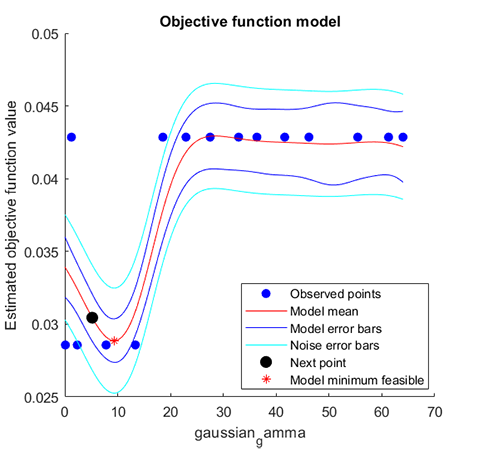
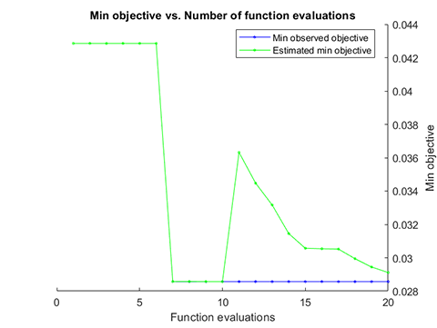
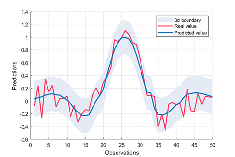
### 06. Parameter Optimization for hybrid-kernel-RVM
A demo for RVM model with Parameter Optimization
```
%{
A demo for hybrid-kernel RVM model with Parameter Optimization
%}
clc
clear all
close all
addpath(genpath(pwd))
% data
load UCI_data
trainData = x;
trainLabel = y;
testData = xt;
testLabel = yt;
% kernel function
kernel_1 = Kernel('type', 'gaussian', 'gamma', 0.5);
kernel_2 = Kernel('type', 'polynomial', 'degree', 2);
% parameter optimization
opt.method = 'bayes'; % bayes, ga, pso
opt.display = 'on';
opt.iteration = 30;
% parameter
parameter = struct( 'display', 'on',...
'type', 'RVR',...
'kernelFunc', [kernel_1, kernel_2],...
'optimization', opt);
rvm = BaseRVM(parameter);
% RVM model training, testing, and visualization
rvm.train(trainData, trainLabel);
results = rvm.test(testData, testLabel);
rvm.draw(results)
```
results:
```
*** RVM model (regression) train finished ***
running time = 24.4042 seconds
iterations = 377
number of samples = 264
number of RVs = 22
ratio of RVs = 8.3333%
RMSE = 0.4864
R2 = 0.7719
MAE = 0.3736
Optimized parameter 1×6 table
gaussian_gamma polynomial_gamma polynomial_offset polynomial_degree gaussian_weight polynomial_weight
______________ ________________ _________________ _________________ _______________ _________________
22.315 13.595 44.83 6 0.042058 0.95794
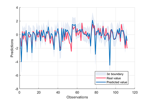
*** RVM model (regression) test finished ***
running time = 0.0008 seconds
number of samples = 112
RMSE = 0.7400
R2 = 0.6668
MAE = 0.4867
```
### 07. Cross Validation
In this code, two cross-validation methods are supported: 'K-Folds' and 'Holdout'.
For example, the cross-validation of 5-Folds is
```
parameter = struct( 'display', 'on',...
'type', 'RVC',...
'kernelFunc', kernel,...
'KFold', 5);
```
For example, the cross-validation of the Holdout method with a ratio of 0.3 is
```
parameter = struct( 'display', 'on',...
'type', 'RVC',...
'kernelFunc', kernel,...
'HoldOut', 0.3);
```
### 08. Other option
```
%% custom optimization option
%{
opt.method = 'bayes'; % bayes, ga, pso
opt.display = 'on';
opt.iteration = 20;
opt.point = 10;
% gaussian kernel function
opt.gaussian.parameterName = {'gamma'};
opt.gaussian.parameterType = {'real'};
opt.gaussian.lowerBound = 2^-6;
opt.gaussian.upperBound = 2^6;
% laplacian kernel function
opt.laplacian.parameterName = {'gamma'};
opt.laplacian.parameterType = {'real'};
opt.laplacian.lowerBound = 2^-6;
opt.laplacian.upperBound = 2^6;
% polynomial kernel function
opt.polynomial.parameterName = {'gamma'; 'offset'; 'degree'};
opt.polynomial.parameterType = {'real'; 'real'; 'integer'};
opt.polynomial.lowerBound = [2^-6; 2^-6; 1];
opt.polynomial.upperBound = [2^6; 2^6; 7];
% sigmoid kernel function
opt.sigmoid.parameterName = {'gamma'; 'offset'};
opt.sigmoid.parameterType = {'real'; 'real'};
opt.sigmoid.lowerBound = [2^-6; 2^-6];
opt.sigmoid.upperBound = [2^6; 2^6];
%}
%% RVM model parameter
%{
'display' : 'on', 'off'
'type' : 'RVR', 'RVC'
'kernelFunc' : kernel function
'KFolds' : cross validation, for example, 5
'HoldOut' : cross validation, for example, 0.3
'freeBasis' : 'on', 'off'
'maxIter' : max iteration, for example, 1000
%}
``` 


